Our approach is to modify several variables to the CGC’s GST calculations to reflect potential future scenarios. Variables impact the final GST amount that states receive in a complex and dynamic way, so this approach can more closely resemble real-world circumstances than a point estimate approach. All publicly available analyses to date have involved modelling based on assumed relativities or scenario-based approaches moving a single variable at a time. This is a new approach to estimating the impacts of the new system of GST.
There are two key steps in implementing this scenario analysis: selecting variables and developing the scenarios. Variable selection in this study involved considering the key drivers of the GST distribution from the CGC’s calculations, ranking them by historical magnitude of impact on the GST distribution and assessing their likely influence on the GST shares. We identified one variable that has a significant impact on the GST distribution, mining royalty revenue, and identified how this interacts with other key drivers. These additional variables were selected based on their relationship with mining royalty revenue.
In the second step, we developed and ran the scenarios. Potential future growth rates of the selected variables were determined by analysing past trends, including how the variables relate to mining royalty revenue. Scenarios were developed by applying past growth rates to forecast future values in line with those trends.
The final set of scenarios focused on the most impactful driver of the GST distribution, mining royalty revenue. Firstly, we conducted a simple analysis to understand its material impacts on the GST distribution. These simple scenarios provided a useful starting point to understand the magnitude of the impact of this one variable. Then we extended this simple analysis using additional variables. The multivariate scenarios are a more realistic modelling approach that incorporates how the variables interact and demonstrates how a particular set of economic conditions can compound the impacts of the new GST system.
The following sections outline the steps we applied to select our variables and implement the multivariate scenario modelling approach to determine the potential fiscal impacts of the new GST system on Victoria.
3.1 Step 1: Selection of variables
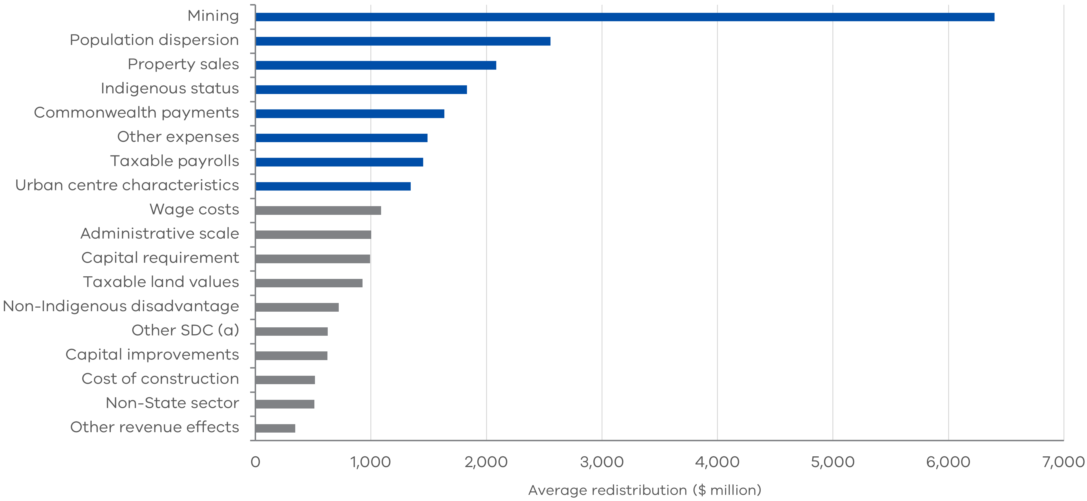
We identified eight variables from the CGC’s assessment method that have been the most impactful in determining states’ final GST relativity and share from 2015–16 to 2021–22. Figure 1 shows the average redistribution of GST according to these variables and the factors of the GST distribution that can have the most influence on a state’s final GST revenue. These variables are also described by the CGC as ‘drivers’ of the GST distribution (CGC 2021).
Of all these variables, mining royalty revenue has the most notable impact on GST distributions by a significant margin. For the period 2015–16 to 2021–22, it had almost as large an impact on the distribution of GST as the next top three drivers combined (population dispersion, property sales and Indigenous status). Not only does it have the largest impact on the CGC’s assessment of relativities, but it also significantly affects the impacts of the new system of GST due to its influence on WA’s GST relativity, as discussed in more detail later in this paper.
The focus on mining royalty revenues targets this work on variables with the most significant impact both independently and when combined. Currently, iron ore is the single most significant commodity impacting the mining revenue assessment, and so we have selected this as a key underlying input to the assessment. As the likelihood of iron ore prices moving in isolation is low, we have constructed multivariate scenarios in addition to just testing the impacts of iron ore prices to capture interactions between other variables. These multivariate scenarios aim to take a more holistic view of potential low, moderate and high iron ore prices, by accounting for other potential flow-on effects to influential components of the GST assessment, like land transfer duty (LTD) and payroll tax.
Figure 1: Drivers of GST and their average redistribution of GST according to assessment category from 2015–16 to 2021–22
Note: (a) Other Sociodemographic Composition includes the effects of age, Indigenous disadvantage, household size, State contributions to the National Disability Insurance Scheme (NDIS) and the full effect of Sociodemographic Composition in Commonwealth funded government schools.
Source: CGC Update Reports, 2015 to 2021.
We exclude other factors presented in Figure 1 from our modelling, generally due to their relatively smaller impact on GST distribution and for ease of modelling and interpretation. Attempting to understand every permutation of variable interaction in the GST system is beyond the scope of this paper.
Variables that were considered but not incorporated into modelling include:
- Commonwealth payments – payments from the Commonwealth other than GST were excluded due to the discretion afforded to the Commonwealth Treasurer and the lack of clear, predictable economic rationale driving payments to underpin modelling.
- Indigenous status – the Indigenous population share of a state and its impact on expenditure requirements was excluded as this variable has remained relatively consistent over time and its interaction with other key variables influencing GST distribution are minimal.
- Urban centre characteristics – this assessment captures the cost of urban transport services for states combining five components: population density, the number of passengers and their mode of transport and distance travelled, topography and the presence of ferry services. This is excluded primarily because the model used for this work is a simplified representation of the CGC’s methods which does not include the level of detail required to alter the sub-components of urban centre characteristics.
3.1.1 Mining revenue
Mining revenue is the single most influential factor determining the redistribution of the GST pool, with over $8 billion set to be redistributed across the states in 2021–22 (CGC 2021). Mining has had an increasing impact on GST distribution since the onset of the mining boom from around 2009 and the expected value of the mining sector in some states has expanded substantially. The CGC’s assessments distribute less GST to states that have strong own-source mining revenues and more GST to states that have less or no capacity to raise mining revenues. This means less GST is distributed to WA and Queensland as they have a higher capacity to raise mining revenues due to greater shares of national natural resources. The CGC’s determination is based on an assessment of the mining production and royalty rate of each commodity.
In 2020–21, mining royalty revenue from WA made up 71 per cent of the total mining royalty revenue of all states, with iron ore comprising 93 per cent. Iron ore makes up a significant portion of the CGC’s mining revenue assessment, and so is considered as the key input for the mining assessment. Iron ore is also among the most volatile of the resources considered by the CGC and its price variability is relatively simple to model.
Higher iron ore prices should increase the impacts of the new system of GST on Victoria, compared to the former system. This is because higher iron ore prices are expected to decrease the GST relativities of resource rich states like WA. If WA has a GST relativity below the relativity floor, or Victoria and NSW’s relativities, GST would be re-distributed from all other states to lift it to these levels. This would leave other states worse off compared to the former system.
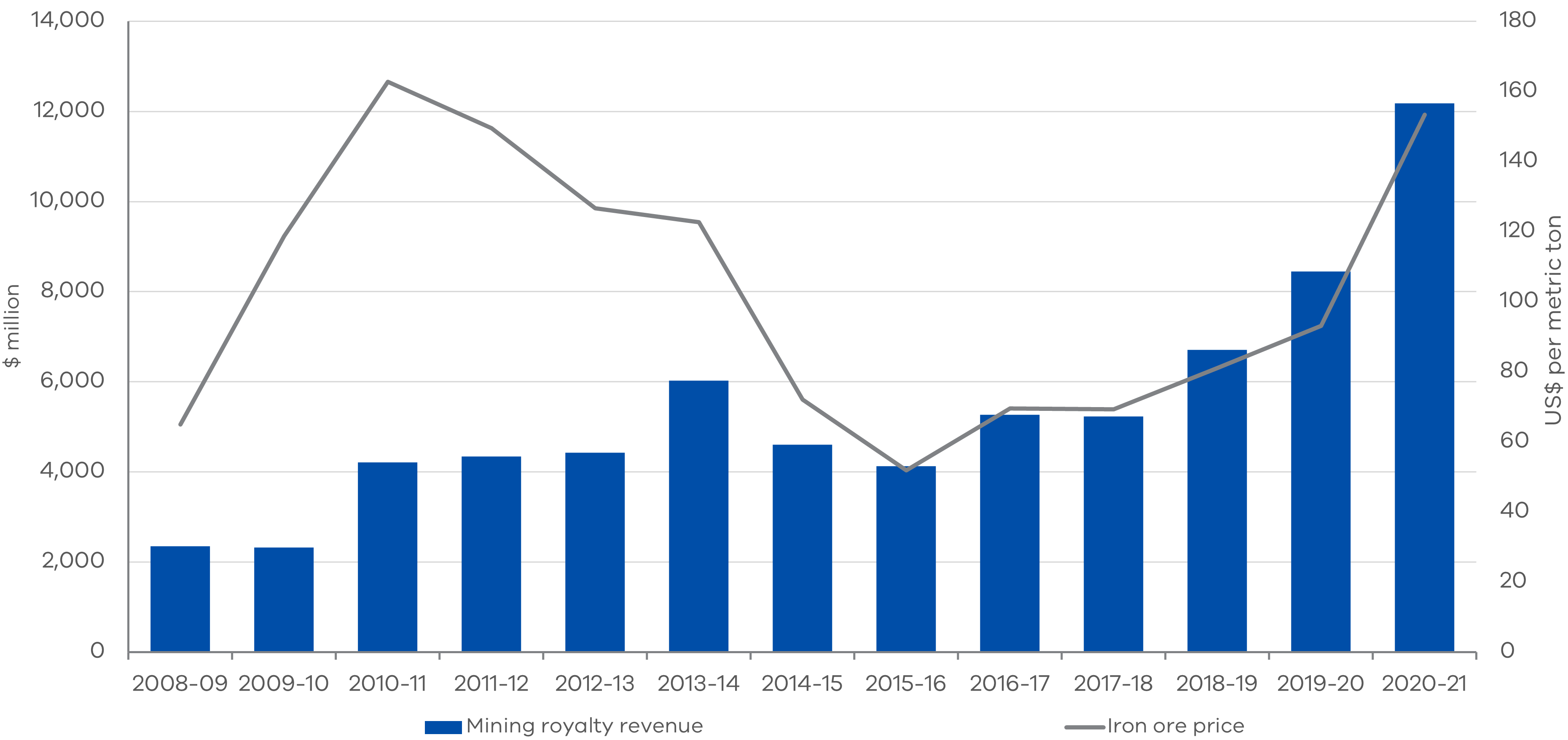
The mining boom and rise of iron ore prices from around 2009 to 2013 significantly affected GST distribution. Figure 2 shows iron ore prices and WA’s royalty revenues peaked around 2010 to 2013 and subsequently declined. Mining royalty revenues closely track iron ore prices. The early divergence between the two can be explained by a 50 per cent royalty rebate provided to iron ore miners in WA until April 2016.
The boom-bust cycles of the resources industry increase the volatility of GST distribution. Through the last mining boom, resource rich states such as WA, Queensland and the NT were assessed to require less GST as they earned more from resource revenues (CGC 2022). As booms end and resource revenues decline, these states then require more GST.
Figure 2: Western Australian mining royalty revenues and the global price of iron ore from 2008-09 to 2020-21
Source: Western Australian budget publications, ABS data, Federal Reserve Bank of St. Louis.
3.1.2 Population dispersion
Population dispersion describes the geographic spread of people and households across the country. The GST system recognises that remote populations cost more to service, so more GST is allocated to states with higher shares of remote populations.
Population dispersion affects the CGC’s assessment of how much it costs a state to provide justice services, post-secondary education, schools and health services, among others. The CGC’s measure of population dispersion uses the Accessibility/Remoteness Index of Australia (ARIA) classifications.
As an example, the NT and Queensland receive a higher share of the GST distribution due to their high incidence of remote populations. In its 2022 update, the CGC estimated that higher shares of remote populations would result in NT and Queensland receiving an additional $1.37 and $1.01 billion more GST than their population shares respectively in 2022–23 (CGC 2022).
3.1.2.1 Population dispersion and mining
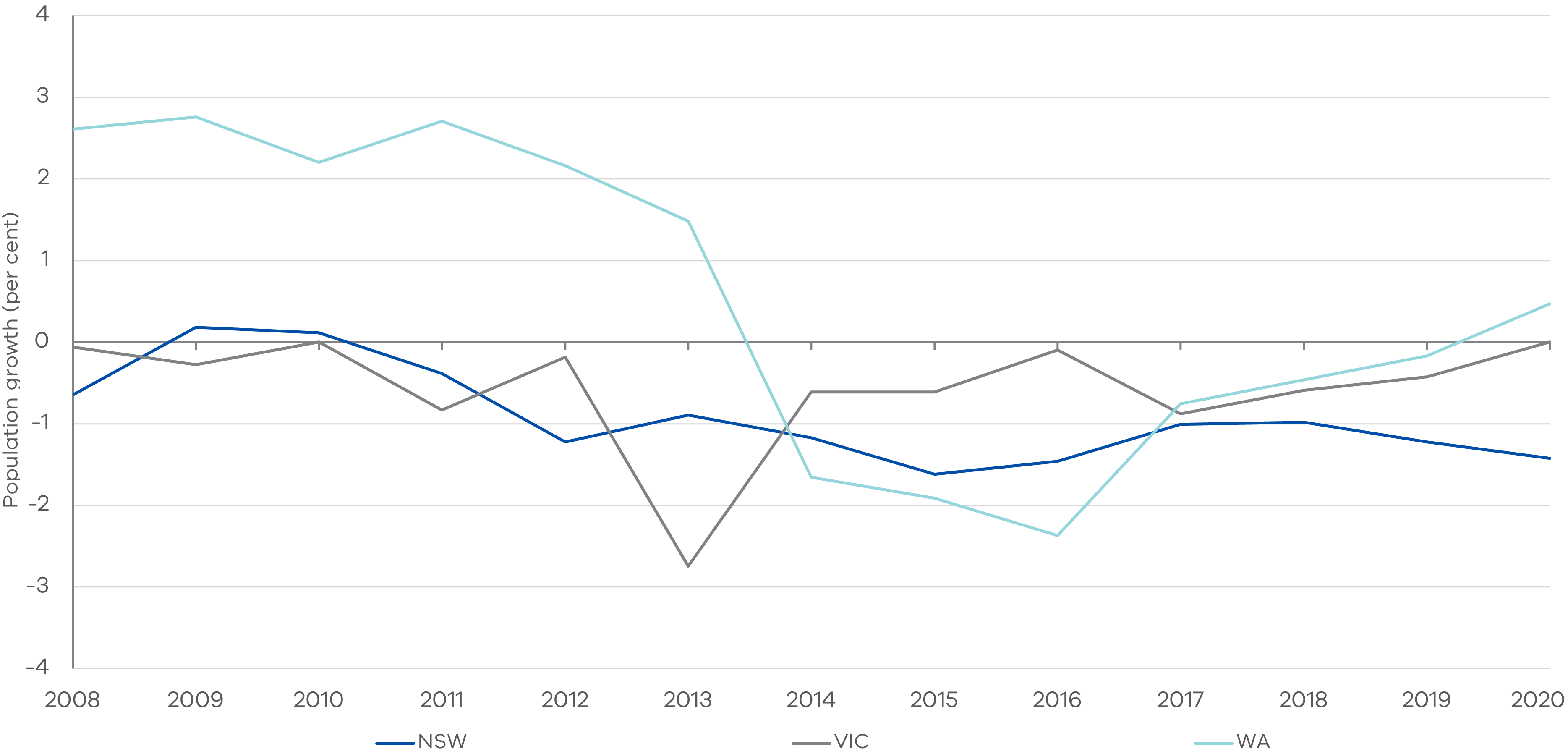
The mining industry has influenced the demographics of remote Australia. The mining boom was linked to population growth in remote mining towns. Due to a low starting base, even a small increase in remote populations can result in relatively large growth rates. For example, the Pilbara region, which produces the largest proportion of WA’s iron ore and is classified as a remote region, saw strong population growth during the mining boom (Garnett 2012). More generally, during the mining boom, population growth for remote and very remote areas in WA was over 2 per cent. When the mining boom slowed, population growth in remote and very remote areas contracted, falling below zero. This is shown in Figure 3 below.
Figure 3: Population growth in remote and very remote areas
Source: ABS, Regional Population 2019–20.
3.1.3 Population growth
While population growth was not identified as a key driver of GST distribution, it is included in the scenarios modelled. This is in part because population growth lends easily to modelling exercises, and because its relationship to changes in mining royalties are clear and can be easily accounted for
Population growth is a direct input into two variables in the GST system – investment and net borrowing – and it also impacts the CGC’s assessment of other expenditures, including states’ base administrative scale costs and services to industry expenses.
The CGC’s Research Paper No. 2 (CGC 2021) explains that the faster the population grows, the more states need to spend on schools, hospitals, roads and other infrastructure. Higher population growth, relative to other states, places a higher investment burden on that state and subsequently increases its GST requirement. Over the past decade, states have experienced varied population growth. This can be decomposed into changes in birth rate, overseas migration or interstate migration. Population growth is both a demand side and supply side factor, linked closely to an increase in economic activity driven by, for example, a mining boom (PM&C 2019)
3.1.3.1 Population growth and mining
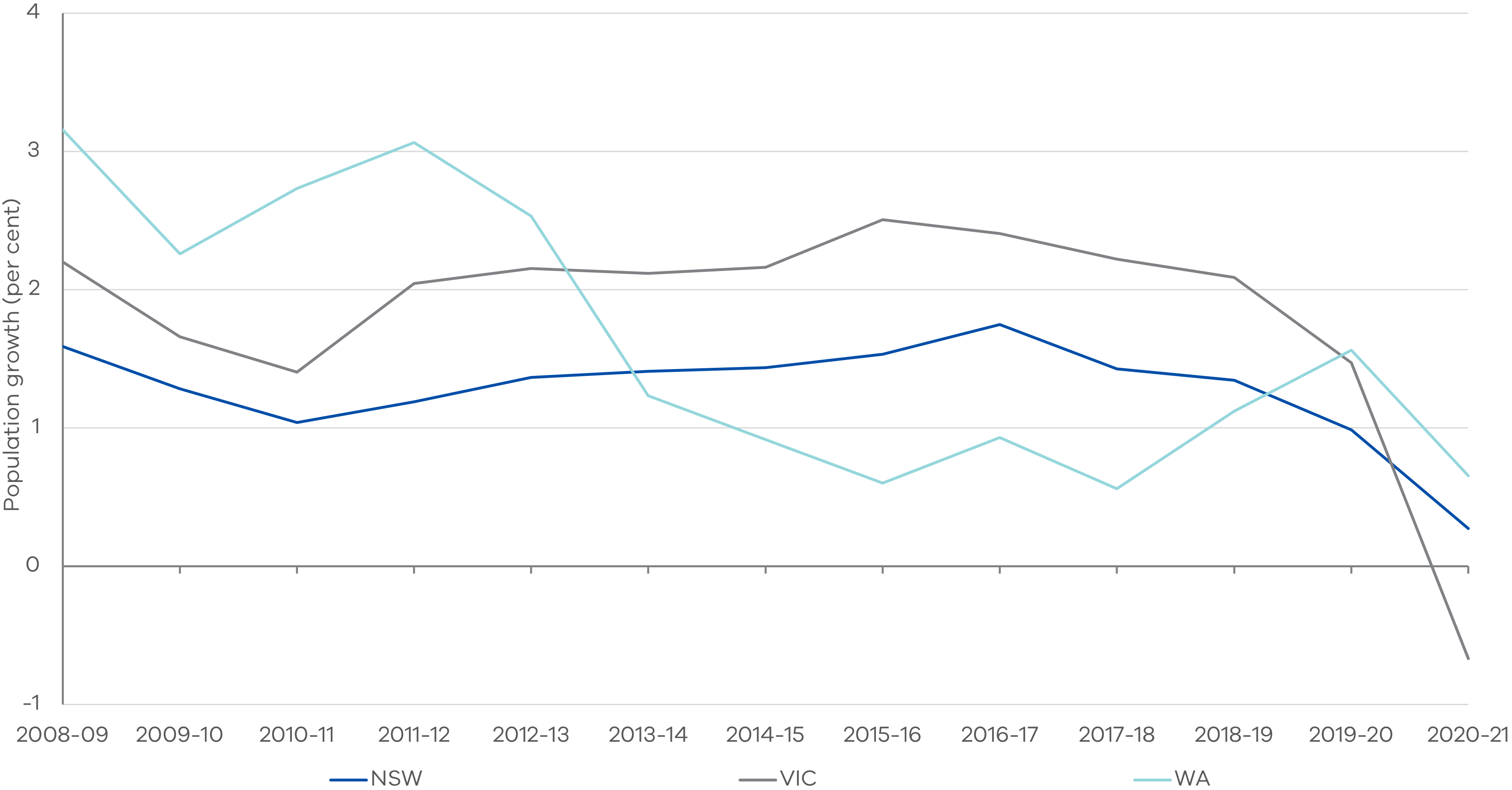
During the mining boom, from around 2008–09 to 2013–14, WA’s population grew more quickly than the populations of NSW and Victoria, averaging over 3 per cent in some years. The boom in WA’s population appears to be related to the circumstances of WA, where the mining industry was experiencing unprecedented growth supported by a rapid increase in overseas migration (Garnett 2012), shown in Figure 4 below. We have incorporated these implied relationships into modelling the impacts of the new system.
Figure 4: Population growth in Victoria, New South Wales and Western Australia from 2008 to 2021
Source: ABS population data.
Note: COVID-19 impacts population growth in 2020–21.
3.1.4 Land transfer duty
Land transfer duty (LTD) is payable on most transactions that result in a change of ownership of land and associated real estate assets in most states. A state’s LTD revenue relies largely on dwelling prices and property transaction volumes. Factors that influence LTD revenue include:
- housing demand, such as from net overseas migration
- credit conditions and mortgage rates
- consumer sentiment towards the housing market.
The CGC assess a state’s capacity to raise LTD by calculating how much it could earn with its tax base, the total value of property transferred and the average tax rate of all states. If a state can earn more LTD than the average state, it will be assessed as requiring relatively less GST.
Revenue from property-based taxes, such as land tax and land transfer duty, is subject to the cyclical movement of property markets, typically related to changes in interest rates and/or changes in sentiment (DTF 2022).
3.1.4.1 LTD and mining
There is some evidence of a positive relationship between mining and LTD revenues for resource rich states like WA. After the mining boom, property prices and LTD revenue declined in WA – house prices in Perth decreased by 20 per cent from June 2014 to December 2020 (Corelogic 2022). In response to recent high iron ore prices, ANZ economists had predicted the average house price in Perth would rise by 12 per cent in 2021 (Emmett and Timbrell 2020).
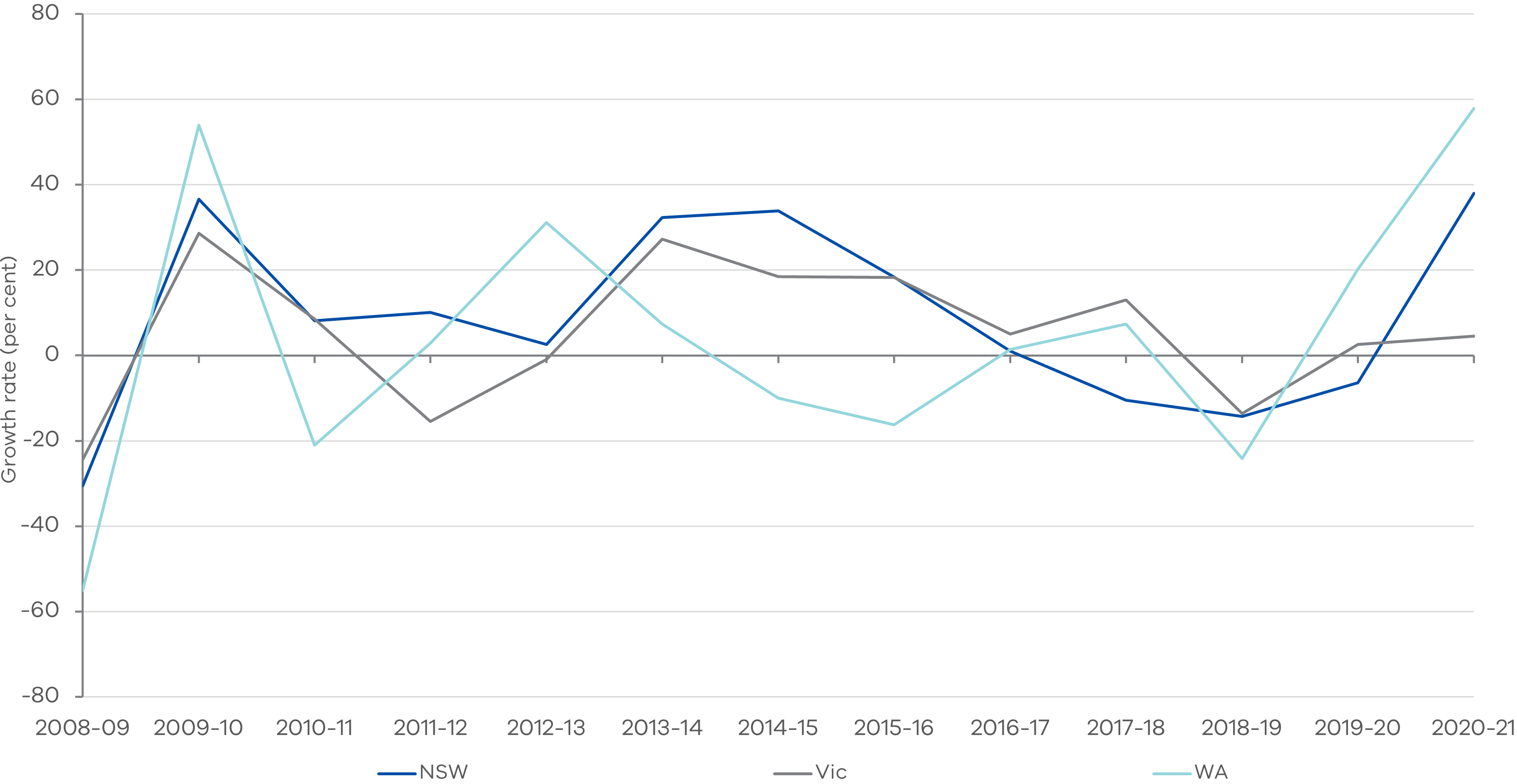
Figure 5 presents the three-year moving average growth rate of LTD. LTD revenue is relatively variable so relationships are less clear, but it shows LTD in WA and the eastern states followed different patterns at different stages of the mining boom. Particularly towards the end of mining boom, after iron ore prices began to fall after 2012–13, growth in LTD revenue in WA fell and was negative from 2014–15 to 2016–17, compared to the eastern states where it continued to grow throughout this period.
Figure 5: Growth rate of stamp duty on conveyances for NSW, Victoria and WA
Source: Victorian, NSW and WA previous state budget papers, 2008–09 to 2021–22.
3.1.5 Payroll tax
Payroll tax is levied by states on the remuneration of employees and is collected by employers for state governments. Across the states, payroll tax is typically applied to businesses with payrolls over a certain threshold and can also vary depending on a business’s total payroll. The CGC assesses states’ capacity to raise payroll tax using their average tax rates and payment thresholds. States with greater capacities to raise their own payroll tax revenues are assessed by the CGC to need less GST revenue.
Payroll tax is based on the total remuneration of employees, which is dependent on states’ macroeconomic conditions. As the economy grows and firms employ more staff or offer higher wages, the payroll tax base and collections also grow (DTF 2021).
3.1.5.1 Payroll tax and mining
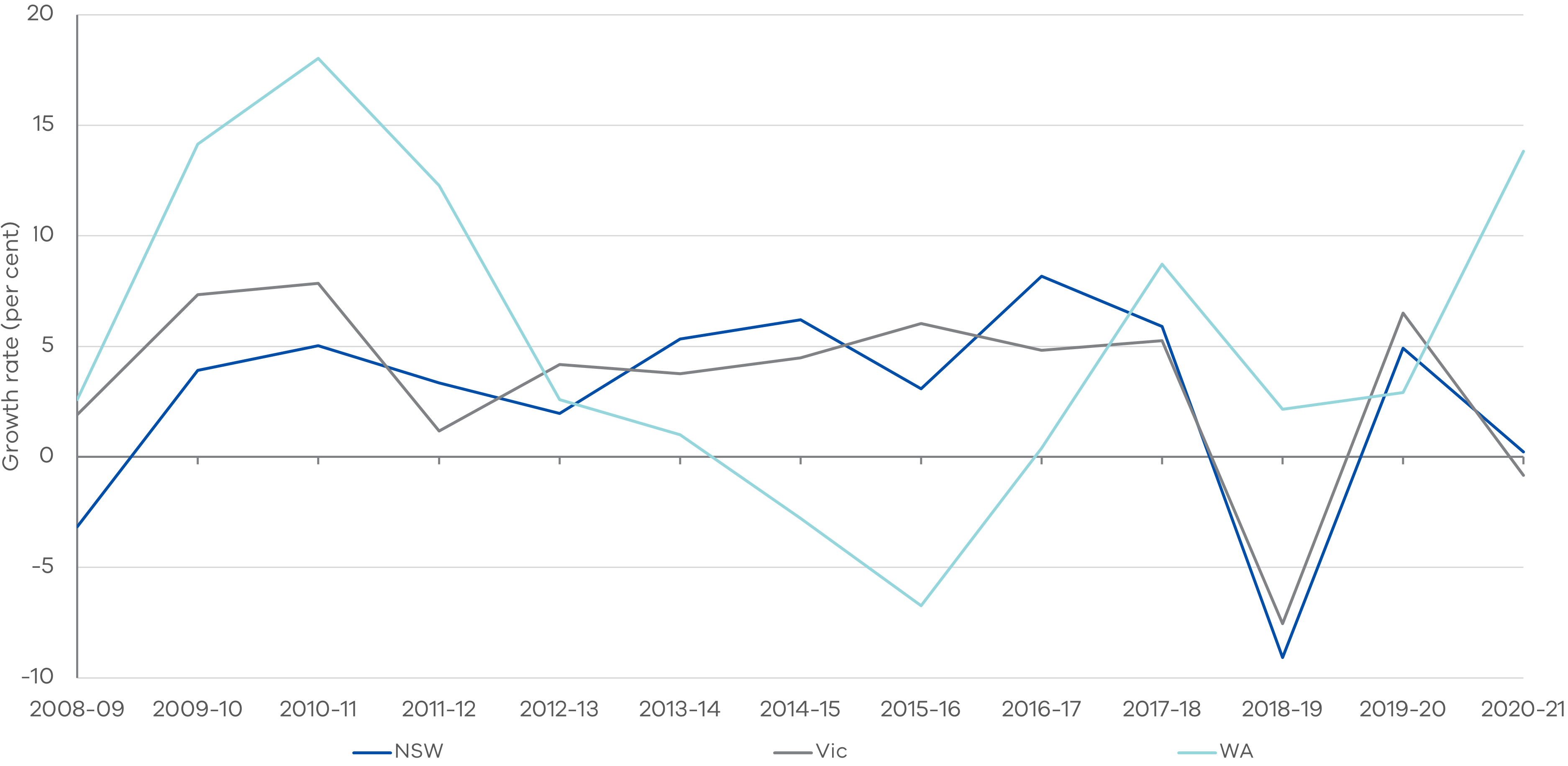
There is some evidence of a positive relationship between mining revenues and payroll tax revenues in resource rich states. In 2013, this was demonstrated by WA in its mining boom, where improved employment and business outcomes are estimated to have raised real wages by 6 per cent and lowered unemployment by about 1.25 percentage points (RBA 2014). This is supported by growth in payroll tax in WA, with the annual growth rate peaking in 2010–11 at almost 20 per cent, demonstrated in Figure 6.
Figure 6: Annual growth rate of payroll tax for NSW, Victoria and WA
Source: Victorian, NSW and WA previous state budget papers, 2008–09 to 2021–22.
3.2 Step 2: Scenario modelling
The scenarios in this paper are estimated through a simplified model of the CGC’s GST formula to arrive at GST relativities and distribution to states. This is done under both the new and former GST systems. The modelling adjusts our selected variables across Victoria, NSW and WA, and measures the corresponding impact on Victoria’s GST share.
The focus of this paper is the impacts of the new system of GST on Victoria, so Victorian variables are modelled in the scenarios. NSW was selected as it is the largest state, but also because it provides the benchmark for the standard of equalisation under the new system along with Victoria. Under the new system, if a state’s GST relativity falls below Victoria and NSW’s then it will be treated as effectively having a lower capacity and requiring more GST. WA was selected due to its significant mining royalty revenues, as mining revenues are the largest driver of the GST distribution. WA is also the state most likely to fall below the GST floor and the new equalisation standard of Victoria and NSW’s relativities. However, other resource rich states such as Queensland may experience similar circumstances to WA in the future if coal prices increase significantly.
The model broadly replicates the CGC’s methods of taking states’ revenue raising capacities and expense burdens to arrive at their GST relativities. There are some key differences, including that our model takes aggregated inputs on states’ spending and revenues from past CGC data. To fully replicate the CGC’s methodology would require comprehensive forecasts for all states that are not available, which is beyond the scope of this article. The CGC’s methodology uses detailed underlying socio-demographic and state budget data, including service use and costs by sub-populations. Every data point would need to be forecast into the long term, which would likely be inaccurate.
Our model estimates the GST revenues Victoria would receive under both the new and former GST systems. The difference between new and former systems for states that are disadvantaged under the new system is equal to the no-worse-off payments they would receive (or very similar, due to the specific calculation of no-worse-off payments).
Scenarios are modelled from 2021–22 to 2026–27. This timeframe aligns with the period of the transition to the new GST system which fully takes effect in 2026–27. Later years are not included primarily due to concerns around the accuracy of forecasting over a longer time horizon.
In developing our scenarios for the period between 2021–22 to 2026–27 we use:
- published actuals and forecasts for revenue and expenses from states’ budget publications
- relativities for past years from the CGC’s relevant final reports
- DTF forecasts of population and the GST pool, based on Commonwealth budget publications.
Using actual values from 2020–21, the selected variables identified in Step 1 are then altered in the model using historical growth rates, with all other variables remaining unchanged.
In addition, this model assumes that the GST methodology remains consistent over the period until 2026–27. We acknowledge that the CGC is expected to complete a methodology review by 2025, potentially impacting 2025–26 and 2026–27.
The multivariate scenarios selected track the impacts of iron ore prices on other variables identified in Step 1 above, including:
- population growth
- population dispersion
- land transfer duty
- payroll tax.
As royalties track iron ore prices, the scenarios use iron ore price forecasts from the Consensus Economics survey of iron ore price as our starting point. Consensus Economics reports prices forecasts from a range of sources and then provide high, low and mean prices in USD per dry metric tonne. The low forecasts are the minimum of all forecasts from their sources and the high forecasts represent the maximum. These price forecasts are used as inputs into our simplified GST model for the period 2021–22 to 2026–27, which then creates projections of mining/iron ore revenue going forward.
3.2.1 Simple scenarios: Moving iron ore prices in isolation
3.2.1.1 Scenario 1a: Low iron ore prices
This scenario is an extremely conservative view of potential iron ore prices, taking the lowest reported iron ore forecasts surveyed by Consensus Economics at time of writing, to understand the impact on Victoria’s GST share.
Iron ore prices are generally forecast by governments and producers to return to low ‘long-run averages’ of around US$60/tonne. In reality, prices fluctuate significantly over time and most organisations caveat long-run forecasts of commodity prices if they are issued at all. The Australian Government Office of the Chief Economist forecasts iron ore prices until 2025, after which they use projections to determine prices.
3.2.1.2 Scenario 2a: Moderate iron ore prices
This scenario takes the mean of iron ore price forecasts surveyed by Consensus Economics and represents a moderate case or our baseline scenario to assess a reasonable outcome.
3.2.1.3 Scenario 3a: High iron ore prices
This scenario takes the highest iron ore forecast price from Consensus Economics. Generally, higher iron ore prices would be expected to reduce Victoria’s GST revenue under the new system compared to the former, as higher iron ore prices are expected to decrease the GST relativity of WA. If WA’s relativity is lower than the legislated floor or Victoria and NSW’s relativity, GST would be re-distributed from other states to lift its relativity, leaving all other states worse off.
3.2.2 Multivariate scenarios: Combining mining prices with other variables
3.2.2.1 Scenario 1b: Low iron ore prices and economic downturn in Western Australia
This multivariate scenario represents the occurrence of a decline in iron ore prices and a decline in economic activity overall. This simulates the effects of decreasing mining revenues combined with the associated decline in economic activity in WA, which holds most of Australia’s iron ore resources.
To simulate this scenario, we have used the low iron ore prices and lower than average growth rates for other own-source revenue streams in WA, including LTD and payroll tax. Population growth and dispersion are assumed to decline due to net migration away from WA as economic opportunities decline.
For NSW and Victoria, the opposite is assumed – population growth is assumed to be high, and growth in LTD and payroll above average.
This scenario assumes the following for each year from 2021–22 to 2026–27:
- 2020–21 actuals as the baseline for growth rates
- ‘low’ iron ore prices obtained from Consensus Economics
- historically low growth rates applied to LTD and payroll revenues, population and population dispersion for WA
- historically high growth rates applied to LTD and payroll revenues, population and population dispersion for Victoria and NSW
- past 10-year average growth rates applied to these variables for all other states.
Growth rates are taken from the period of 2013–14 to 2016–17, relating to the waning of the mining boom in WA.
3.2.2.2 Scenario 2b: Moderate iron ore prices and long-term growth rates for other variables
This multivariate scenario tests what would occur if all states experienced growth in the selected variables in line with 10-year average growth rates. This scenario relates to a ‘status quo’ generally continuing until the end of the transition period in 2026–27.
This smooths out peaks or troughs in economic circumstances and is useful for understanding the impacts of median forecast iron ore prices with similarly moderate outcomes for LTD, payroll tax and population growth. This scenario does not adjust levels of population dispersion and assumes current trends continue as a baseline.
3.2.2.3 Scenario 3b: Economic boom in WA and unfavourable conditions in eastern states
This multi-variable scenario tests the impacts of high iron ore prices and the potential flow on effects to the other selected variables, representing an economic boom in WA and the inverse in eastern states. Historically, high iron ore prices have increased economic activity in WA due to its concentration of iron ore resources. Population growth and population dispersion in WA are assumed to grow strongly. This simulates movement of people taking advantage of economic opportunities and relocating to remote areas servicing the resources industry.
This is coupled with the opposite occurring in NSW and Victoria. A resources boom in WA is assumed to cause migration away from the eastern states, decreasing population growth. This also results in lower own-source revenues for these states.
More specifically, this scenario assumes the following for each year from 2021–22 to 2026–27:
- high iron ore prices from Consensus Economics
- 2020–21 actuals as the baseline for relevant growth rates
- historically high growth rates applied to LTD and payroll revenues, population and population dispersion for WA
- historically low growth rates applied to LTD and payroll revenues, population and population dispersion for Victoria and NSW
- past 10-year average growth rates applied to these variables for all other states.
Growth rates are taken from the period of the mining boom between 2009 to 2013, which was a time of high economic growth in WA.
Updated


